
Logistic Regression Implementation using Python
Logistic Regression
Basic Assumptions:
1) target variable y is binary and follows Bernoulli distribution
2) independent variable should have little or no collinearity
3) linearly related to the log odds
4) should have sufficient amount of data
5) Model parameters are estimated using gradient descent or Max Conditional Likelihood estimation
Problem Statement
The objective is to predict whether an individual will default on his credit card payment, on the basis of his bank balanc, income and whether he is a student or not
Dataset can be downloaded from here.
A simulated data set containing information on ten thousand customers.
import pandas as pd
import numpy as np
import matplotlib.pyplot as plt
!pip install xlrd
org_data = pd.read_excel("LogisticRegressionDemo.xlsx")
Requirement already satisfied: xlrd in c:\users\i330087\appdata\local\continuum\anaconda3\lib\site-packages (1.2.0)
#org_data = org_data.drop(['Unnamed: 0'], axis=1)
org_data.head()
| Unnamed: 0 | default | student | balance | income | |
|---|---|---|---|---|---|
| 0 | 1 | No | No | 729.526495 | 44361.625074 |
| 1 | 2 | No | Yes | 817.180407 | 12106.134700 |
| 2 | 3 | No | No | 1073.549164 | 31767.138947 |
| 3 | 4 | No | No | 529.250605 | 35704.493935 |
| 4 | 5 | No | No | 785.655883 | 38463.495879 |
# check the data set dimensions and obtain basic information. <br> shape attribute provides data size i.e. no of obs as rows and no. of features as columns.<br>
# describe function provides statistical summary
print(org_data.shape)
org_data = org_data.drop(['Unnamed: 0'], axis=1)
org_data.info()
# Try org_data.describe() for printing the statistical summary
(10000, 5)
<class 'pandas.core.frame.DataFrame'>
RangeIndex: 10000 entries, 0 to 9999
Data columns (total 4 columns):
default    10000 non-null object
student    10000 non-null object
balance    10000 non-null float64
income     10000 non-null float64
dtypes: float64(2), object(2)
memory usage: 312.6+ KB
Notice that there are no missing values in the dataset. All columns have non-null values
Print the number of positive and negative instances
print(org_data.default.value_counts())
No     9667
Yes     333
Name: default, dtype: int64
A heavily class imbalanced problem with only 3.5% non-defaulters
data = org_data[['default',"student",'balance','income']]
data = data[1:1000]
print(data.shape)
data.default.value_counts()
#data.head()
(999, 4)


No     961
Yes     38
Name: default, dtype: int64
Since the response variable “default” and the predictor student have categorical values in the form of “yes” and “no”, it is important to encode them using 0/1 form to feed as input to the model.
factorize() method is used to perform this conversion
data['default'],default_unique = data['default'].factorize()
data['student'], st_unique = data['student'].factorize()
print("unique student labels",st_unique)
print("unique default labels",default_unique)
data.head()
unique student labels Index(['Yes', 'No'], dtype='object')
unique default labels Index(['No', 'Yes'], dtype='object')
| default | student | balance | income | |
|---|---|---|---|---|
| 1 | 0 | 0 | 817.180407 | 12106.134700 |
| 2 | 0 | 1 | 1073.549164 | 31767.138947 |
| 3 | 0 | 1 | 529.250605 | 35704.493935 |
| 4 | 0 | 1 | 785.655883 | 38463.495879 |
| 5 | 0 | 0 | 919.588530 | 7491.558572 |
This implies that student=’Yes’ is encoded as 0 and student=’No’ is encoded as 1. Similarly, default=’No’ is encoded as 0 and default=’yes’ as 1.
data.corr()
| default | student | balance | income | |
|---|---|---|---|---|
| default | 1.000000 | -0.018135 | 0.360888 | 0.014253 |
| student | -0.018135 | 1.000000 | -0.227472 | 0.755412 |
| balance | 0.360888 | -0.227472 | 1.000000 | -0.137466 |
| income | 0.014253 | 0.755412 | -0.137466 | 1.000000 |
the highest correlation between default and the other predictors is with Balance. Thus, balance has strong infulence on whether the candidate will default on his credit payment or not. The correlation beween student and income is much lesser.
student has negative correlation with default i.e. chances of a student defaulting is lesser than that of a non-student defaulting. Also notice the high positive correlation between student and income, negative correlation between student and balance.
It will be good to explore this for different subsets and then the entire dataset to notice the change in these correlation coefficients and observe true relatinship
Visualize relationship between response vs predictors
The response variable for a binary linear regression problem has only two options: 0/1, creating a scatter plot is not helpful here. Instead, box plots and contingency tables provide good understanding of the data.
pd.crosstab(data.student, data.default).plot(kind='bar')
<matplotlib.axes._subplots.AxesSubplot at 0x255e04307b8>
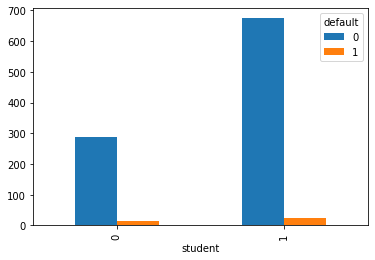
Is student a good indicator of defaulter? For defaulter = NO, i.e. non-deafulters, the difference between student=yes(0) and non-student is very prominent i.e. chances of student defaulting is much less than the chances of non-students defaulting. But for defaulters, the distinction is not that significant.
# boxplot
data.boxplot(column='balance',by='default')
<matplotlib.axes._subplots.AxesSubplot at 0x255e069c9b0>
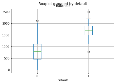
The purpose of visualization is to think about questions such as: What does this bar chart or box plot convey?
There is a huge difference in balance between defaulters and non-defaulters.
Check for income vs default as well.
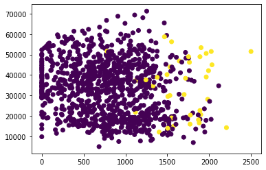
Another visualization style in practice is to see relationship between predictors and response using coloured scatter plots as follows
plt.scatter(data.balance, data.income, c=data.default)
<matplotlib.collections.PathCollection at 0x255e05ac940>
from sklearn.linear_model import LogisticRegression
from sklearn.metrics import accuracy_score
from sklearn.model_selection import train_test_split
model1 = LogisticRegression()
# X = data.balance.values.reshape(-1,1)
#X = data[['balance','student']]
X = data[['balance','student','income']]
# print(X.shape)
y = data.default.values.reshape(-1,1)

x_train, x_test, y_train, y_test = train_test_split(X,data.default,test_size=0.20,random_state=105)
model1.fit(X, y)
C:\Users\I330087\AppData\Local\Continuum\anaconda3\lib\site-packages\sklearn\linear_model\logistic.py:432: FutureWarning: Default solver will be changed to 'lbfgs' in 0.22. Specify a solver to silence this warning.
  FutureWarning)
C:\Users\I330087\AppData\Local\Continuum\anaconda3\lib\site-packages\sklearn\utils\validation.py:724: DataConversionWarning: A column-vector y was passed when a 1d array was expected. Please change the shape of y to (n_samples, ), for example using ravel().
  y = column_or_1d(y, warn=True)


LogisticRegression(C=1.0, class_weight=None, dual=False, fit_intercept=True,
                   intercept_scaling=1, l1_ratio=None, max_iter=100,
                   multi_class='warn', n_jobs=None, penalty='l2',
                   random_state=None, solver='warn', tol=0.0001, verbose=0,
                   warm_start=False)
print('classes: ',model1.classes_)
print('coefficients: ',model1.coef_)
print('intercept :', model1.intercept_)
classes:  [0 1]
coefficients:  [[ 2.30714566e-04  3.36201089e-07 -1.09177044e-04]]
intercept : [-1.43338127e-06]
Model Equation \begin{equation} z = 2.30714566e-04balance + 3.36201089e^{-07} * student - 1.091e^{-04}income \end{equation}
\begin{equation} sigma(z) = \frac{1}{ 1+e^{-z}} \end{equation}
# test1={'balance':40, 'student':1,'income':1500}
# x_test = pd.DataFrame(test1, index=[0])
predictions = model1.predict(x_test)
#print(predictions)
score = accuracy_score(predictions, y_test)
print(score)
0.945
from sklearn import metrics
print("prediction shape",predictions.shape)
print("y_test.shape", y_test.shape)
cm = metrics.confusion_matrix(predictions, y_test)
print(cm)
prediction shape (200,)
y_test.shape (200,)
[[189  11]
 [  0   0]]
# Predicting for an unknown test case
test1={'balance':3000, 'student':1,'income':1500}
x_test1 = pd.DataFrame(test1, index=[0])
predictions = model1.predict(x_test1)
print(predictions)

prob = model1.predict_proba(x_test1)
print(prob)
[1]
[[0.3708955 0.6291045]]
How do you interpret the result?
The sklearn model doesnot provide statistical summary to help us understand which features are not relevant and can be removed.
Statsmodel provides a good alternative to this and provides a detailed statistical summary that helps in feature selection as well.
model2 = LogisticRegression()
X2 = data[['student']]
y2 = data[['default']]
model2.fit(X2, y2)
C:\Users\I330087\AppData\Local\Continuum\anaconda3\lib\site-packages\sklearn\linear_model\logistic.py:432: FutureWarning: Default solver will be changed to 'lbfgs' in 0.22. Specify a solver to silence this warning.
  FutureWarning)
C:\Users\I330087\AppData\Local\Continuum\anaconda3\lib\site-packages\sklearn\utils\validation.py:724: DataConversionWarning: A column-vector y was passed when a 1d array was expected. Please change the shape of y to (n_samples, ), for example using ravel().
  y = column_or_1d(y, warn=True)


LogisticRegression(C=1.0, class_weight=None, dual=False, fit_intercept=True,
                   intercept_scaling=1, l1_ratio=None, max_iter=100,
                   multi_class='warn', n_jobs=None, penalty='l2',
                   random_state=None, solver='warn', tol=0.0001, verbose=0,
                   warm_start=False)
print(model2.coef_)
print(model2.intercept_)
test2 = {'student':1}
x_test2 = pd.DataFrame(test2, index=[0])
model2.predict(x_test2)
prob = model2.predict_proba(x_test2)
print(prob)
[[-0.37162045]]
[-2.90741904]
[[0.9637027 0.0362973]]
Contrasting results: model 1 predicts the prob of a studen defaulting is higher than non-defaulting whereas model 2 predicts the chance ofa student defaulting is much higehr.
from statsmodels.api import OLS
OLS(data.default,X).fit().summary()
| Dep. Variable: | default | R-squared (uncentered): | 0.138 |
|---|---|---|---|
| Model: | OLS | Adj. R-squared (uncentered): | 0.135 |
| Method: | Least Squares | F-statistic: | 52.98 |
| Date: | Sat, 14 Dec 2019 | Prob (F-statistic): | 8.92e-32 |
| Time: | 14:32:04 | Log-Likelihood: | 289.39 |
| No. Observations: | 999 | AIC: | -572.8 |
| Df Residuals: | 996 | BIC: | -558.1 |
| Df Model: | 3 | ||
| Covariance Type: | nonrobust |
| coef | std err | t | P>|t| | [0.025 | 0.975] | |
|---|---|---|---|---|---|---|
| balance | 0.0001 | 1e-05 | 10.750 | 0.000 | 8.82e-05 | 0.000 |
| student | 0.0215 | 0.019 | 1.103 | 0.270 | -0.017 | 0.060 |
| income | -1.666e-06 | 5.38e-07 | -3.095 | 0.002 | -2.72e-06 | -6.1e-07 |
| Omnibus: | 878.203 | Durbin-Watson: | 1.838 |
|---|---|---|---|
| Prob(Omnibus): | 0.000 | Jarque-Bera (JB): | 16270.196 |
| Skew: | 4.239 | Prob(JB): | 0.00 |
| Kurtosis: | 20.861 | Cond. No. | 1.22e+05 |
Warnings:
[1] Standard Errors assume that the covariance matrix of the errors is correctly specified.
[2] The condition number is large, 1.22e+05. This might indicate that there are
strong multicollinearity or other numerical problems.
NOTE Remember we had observed high correlation between student and income. Important to notice the p-values for each of the coefficients. The t-statistics of student [P>|t|] is a very high value and we need to accept the hypothesis tht student has no relation with default and this is one feature that can be removed from consideration.
from sklearn.naive_bayes import GaussianNB
gnb_model = GaussianNB()
gnb_model.fit(x_train, y_train)
GaussianNB(priors=None, var_smoothing=1e-09)
gnb_predictions = gnb_model.predict(x_test)
#print(gnb_predictions.shape)
#print(y_test.shape)
score = accuracy_score(gnb_predictions, y_test)
print("Gaussian NB accuracy : ", score)
Gaussian NB accuracy : 0.96
gnb_model.class_prior_
array([0.96620776, 0.03379224])
For the current test case, the probability of defaulter (class=0) is much higher than that of a non-defaulter.
NOTE: For the current subset of data, performance of GNB is better than that of Logistic regression because the training data set is of limited size. Try testing it on the whole dataset and then compare the performance.